09.02.2017 by Infogram
Google Sheets is a great free tool for creating and editing spreadsheets. It allows you to easily work in real time and collaborate with others. Google Sheets has a lot of features you may not be familiar with that are guaranteed to make you more productive.
In this article, we’ll share 17 Google Sheets tips and tricks that will help save you time at work. Keep reading if you want to learn how to make the most of your data, in less time:
- Keyboard shortcuts
- Add images to cells
- Use SQL commands and the query function
- Extract only the date portion of a timestamp
- Create QR codes
- Create live charts with Infogram
- Lookup values based on multiple criteria
- Use the FILTER() function
- Get only unique values from a column
- Web scraping with Google Sheets
- Detect a language
- Translate a language
- Check for valid emails and URLs
- Project future results with GROWTH()
- Make your formulas easier to read
- Add funky characters to your spreadsheet
- Pick randomly from a list
1) Keyboard shortcuts
You may know a few shortcuts like copy and paste (Ctrl + C, Ctrl + V) but there are more powerful commands at your fingertips. Shortcuts that let you move to the next sheet and change data formats, for example.
Locate the ‘Help’ menu to learn a few more or check out this list of keyboard shortcuts.
2) Add images to cells
To place an image straight into a cell type =image(“URL of the image you want to add”). There are a few options for inserting and formatting images:
- =image(“URL of the image”,1) – image scaled to fit the cell
- =image(“URL of the image”,2) – image stretched to fit the cell
- =image(“URL of the image”,3) – image keeps its original size
- =image(“URL of the image”,4) – image in a custom size
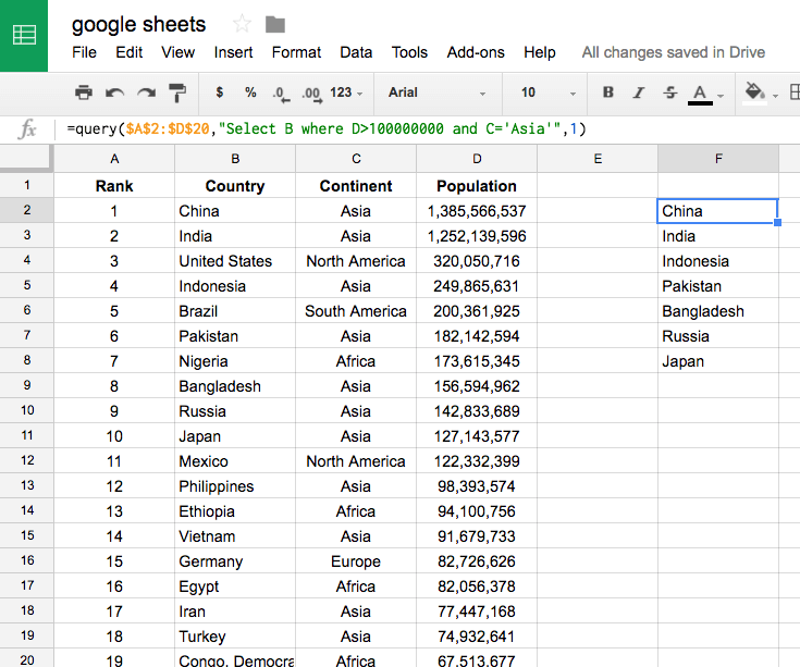
3) Use SQL commands and the query function
Take advantage of the QUERY( ) function in Google Sheets to start treating your tables like databases where you can retrieve any figure based on SQL code.
Query offers all the capabilities of arithmetic functions (SUM, COUNT, AVERAGE) with the filtering abilities of a function like FILTER. To learn more we recommend this article.
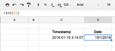
4) Extract only the date portion of a timestamp
If you have timestamps in your spreadsheet there is an easy way to remove the time data. Use the INT( ) function to extract only the date portion of a timestamp.
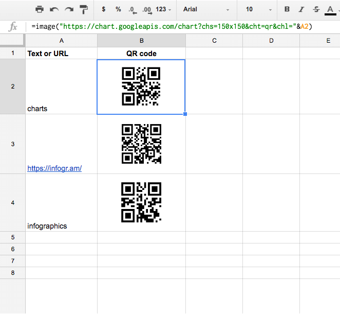
5) Create QR codes
QR codes can be used for a number of reasons – including WiFi login, concert tickets, advertisements, and product purchases. Google Sheets lets you generate QR codes with any input you like. Just use the following formula:
=image(“https://chart.googleapis.com/chart?chs=150×150&cht=qr&chl=”&A2).
A2 is the cell with the URL or text you want to use to create your QR code.
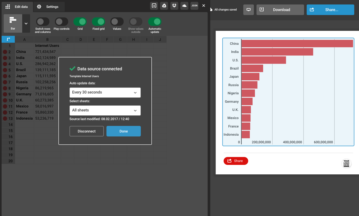
6) Create live charts with Infogram
Infogram’s integration with Google Sheets automates the process of adding new data to a chart by updating the data periodically. It is simple to set up, so you might want to try it when designing your next interactive chart or online report. View the tutorial here.
Would you like to experience the full power of data visualization? Try Infogram for Teams or Enterprise for free! With a Team or Enterprise account, you can create up to 10,000+ projects, collaborate with your team in real time, use our engagement analytics feature, and more. Request your free demo here.
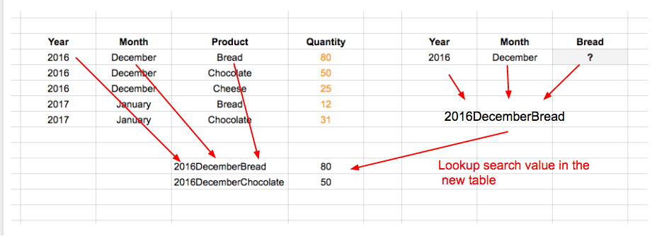
7) Lookup values based on multiple criteria
You may be aware of lookup functions (VLOOKUP or INDEX/MATCH) that allow you to search based on one term. If you want to search using multiple criteria you can use the ARRAYFORMULA function. Here’s an example, using this formula:
=ARRAYFORMULA(index($E$4:$E$8,match($G4&$H4&$I$3,$B$4:$B$8&$C$4:$C$8&$D$4:$D8,0)))
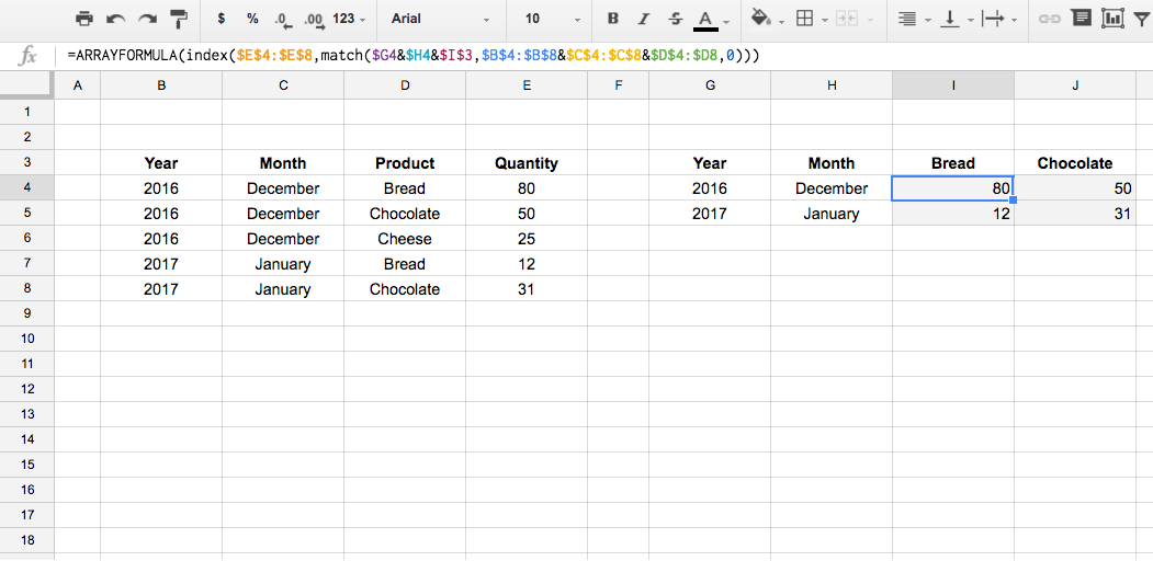
The diagram below explains how the formula works. Learn more here.
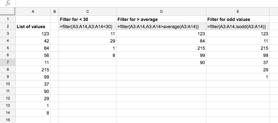
8) Use the FILTER( ) function
The FILTER function allows you to easily return values from a column that satisfy certain conditions. FILTER can only be used to filter rows or columns at one time.
The syntax is: =FILTER(“list of values”, “conditions we’re testing”).
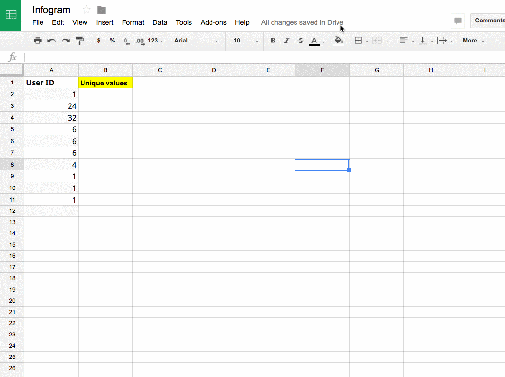
9) Get only unique values from a column
Use the function UNIQUE( ) to get a list of unique values from a range or column.
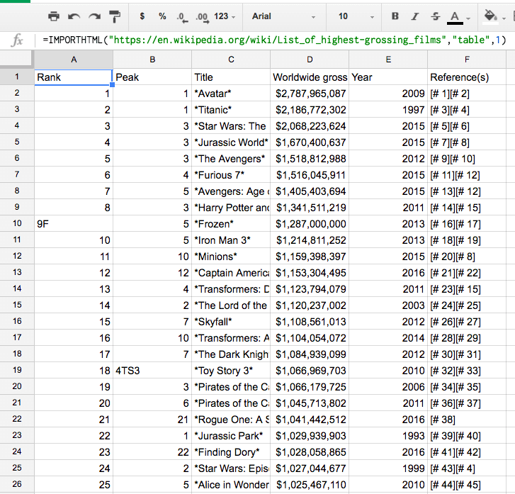
10) Web scraping with Google Sheets
You can access data from a website in your spreadsheet without having to copy and paste using the IMPORTHTML( ) or IMPORTXML( ) functions.
Copy the formula below into A1 and you’ll see the same data as the image below:
=IMPORTHTML(“https://en.wikipedia.org/wiki/List_of_highest-grossing_films”,”table“,1)
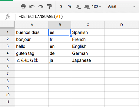
11) Detect a language
Google has a built-in language detector. Use the formula DETECTLANGUAGE( ) and it will return a two letter language code. The full list of language codes can be found here.
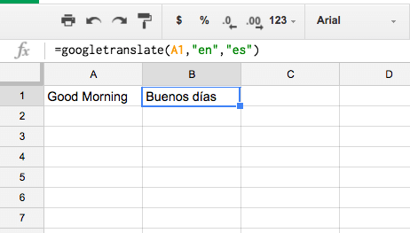
12) Translate a language
Google can detect a language but also translate from one language to another.
The formula GOOGLETRANSLATE( ) has three parts – text to translate, the current language of the text, and the language you want to translate into.
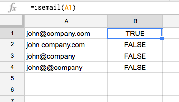
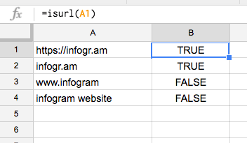
13) Check for valid emails and URLs
The function ISEMAIL( ) checks to see if a string of text or cell has a valid email syntax.
The function ISURL( ) returns true or false if a string of text or cell has a valid URL.
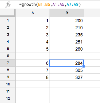
14) Project future results with GROWTH( )
The GROWTH( ) function can be used to extrapolate a trend and predict future values.
The image below shows the sales of a product over 5 periods. With the formula =growth(B1:B5,A1:A5,A7:A9) you can estimate what the values would be for 6 – 8.
15) Make your formulas easier to read
Have a long formula? Break it into easy to read lines using the command ALT + Enter.
Before using the formula:
=IF(( SUMIF(A2:A20,”SOLD”,B2:B20)) > 2000,”More than $1000 SOLD”,”Less than $100 SOLD”)
After using ALT + Enter:
=IF( ( SUMIF(A2:A20,”SOLD”,B2:B20)) > 2000,
“More than $2000 SOLD”,
“Less than $200 SOLD” )
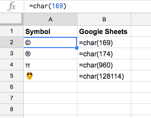
16) Add funky characters to your spreadsheet
The CHAR( ) function lets you insert symbols like trademark ©, copyright ® or the number pi π. To find interesting symbols we recommend Graphemica.
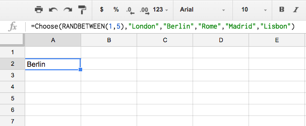
17) Pick randomly from a list
The functions CHOOSE( ) AND RANDBETWEEN( ) help you pick a value from a defined list. RANDBETWEEN( ) generates a random integer between 1 and 5. CHOOSE( ) helps you pick from the list of entries.
=CHOOSE(RANDBETWEEN(1,5),”London”,”Berlin”,”Rome”,”Madrid”,”Lisbon”)
We hope these tricks boost your productivity and make you a Google Sheets master. If you found these tips useful, pass this article along to your colleagues & friends! You can also read about 5 ways how to fix your bad data
<
p style=”text-align: center;”>
Get data visualization tips every week:
New features, special offers, and exciting news about the world of data visualization.